Data

The dataset employed regards the counts of accesses to gender-based violence support centers in the Apulia region by residence municipality of the women victims of violence during 2022. R codes to generate the dataset are in the R script posted here which this report is based on.

Here, we only take into account the violence reports which support centers actually take charge of, at the risk of underestimating the counts of gender-based violence cases. This choice is driven by the need of avoiding duplicated records, since e.g. it may happen that a support center redirects a victim to another support center.

In order to avoid singletons in the spatial structure of the dataset, we removed the Tremiti Islands from the list of municipalities included (\(0\) accesses to support centers in 2022).

Therefore, the municipality-level dataset in scope consists of \(256\) observations.

We can only take into account the accesses to support centers for which the origin municipality of victims is reported. Therefore, the total count of accesses in scope is \(2259\). Among these accesses, \(1516\) were taken charge of.

Here, we plot the log-access rate per residence municipality, i.e. the logarithm of the ratio between access counts and female population. Blank areas correspond to municipalities from which zero women accessed support centers (\(82\) municipalities).

Covariates

Our target is explaining the number of accesses to support centers, \(y\), defined at the municipality level, on the basis of a set of candidate known variables.

We model \(y\) via a simple Poisson GLM.

We have at disposal a number of candidate explanatory variables, which include the distance of a municipality from the closest support center and a set of variables measuring social vulnerability under different dimensions; these latter covariates are provided by the ISTAT.A more detailed description of these covariates is in this excel metadata file.

All covariates are scaled to have null mean and unit variance.

For instance, the support center designated for the municipality of Adelfia (province of Bari, \(3\)rd municipality in the dataset) is located in Capurso (BA). Then, \(\mathrm{TEP}_{3}\) denotes the travel time between Adelfia and Capurso (\(17\) minutes).

First, we visualise the correlations among these explanatory variables:

We see the correlation between the two distances is very high (\(0.72\)), and so is the correlation between the fragility index decile and the density of productive units.

In the first case, we drop the distance from the nearest infrastructural pole We do so because, if taken alone, the distance from the closest support center appears a slightly better predictor, using the Schwarz information criterion (or, indifferently, the Akaike Information Criterion):

stats::BIC(glm(N_ACC ~ 1 + AES, family = "poisson",
               offset = log(nn), data = dd_con))
## [1] 1124.922
stats::BIC(glm(N_ACC ~ 1 + TEP_th_22, family = "poisson",
               offset = log(nn), data = dd_con))
## [1] 1120.389

We should do the same for the other couple of variables but since MFI is a combination of all covariate except for TEP_th, we will drop the synthetic indicator and leave the remainder.

Nonspatial regression

We regress the counts of accesses \(y\) to support centers on the aforementioned explanatory variables. To estimate regression coefficients, all covariates are scaled to zero mean an unit variance.

\[\begin{equation} y_i \mid \eta_i \sim \mathrm{Poisson}(E_i \, e^{\eta_i}) \quad \text{where} \quad \eta_i = X_i^{\top} \alpha \label{eq:glm} \end{equation}\]

Where \(X\) are the covariate defined earlier, \(\alpha\) are covariate effects, and \(E_i\) is the female population aged \(> 14\) in municipality \(i\).

To gain more insight on the role of all explanatory variables we show the posterior summaries of the full regression model

cav_glm <- glm(N_ACC ~ 1 +TEP_th_22 + ELI + PGR +
                 UIS + ELL + PDI + ER,
               family = "poisson",offset = log(nn), data = dd_con)
summary(cav_glm)$coefficients
##                Estimate Std. Error     z value     Pr(>|z|)
## (Intercept) -7.46748635 0.04524877 -165.031813 0.000000e+00
## TEP_th_22   -0.39714306 0.04201946   -9.451407 3.343054e-21
## ELI         -0.07087461 0.03369481   -2.103428 3.542838e-02
## PGR          0.12914911 0.04270159    3.024457 2.490801e-03
## UIS         -0.09776366 0.03510686   -2.784745 5.356979e-03
## ELL         -0.11515036 0.04427412   -2.600851 9.299292e-03
## PDI         -0.06869493 0.04521827   -1.519185 1.287159e-01
## ER          -0.06640563 0.05019652   -1.322913 1.858643e-01

How do we interpret the size of regression coefficient of TEP_th_22? Keeping in mind we are working on the logarithm of the access rate, the standard deviation of the distance, expressed in minutes, is:

# Distance from closest support center
attr(scale(dists_th_22$TEP_th_22), "scaled:scale")
## [1] 14.10021

Hence e.g. each \(14'6''\) of distance of the a given municipality from the closest support center are associated with a decrease of \(0.399\) units in the log-frequency at which women from that municipality access to support centers.

Additionally, the number of zero counts is high:

sum(dd_con$N_ACC == 0)
barplot(table(dd_con$N_ACC))

We may wonder if the data generating process incorporates a zero-generating component. We can model this augmented process through zero-inflated Poisson likelihood: \[ p(y_i | \eta_i) = \pi_0 \mathbb{I}{ \lbrace y_i=0 \rbrace } + (1-\pi_0) \frac{ e^{-E_i e^{\eta_i } +(\ln E_i + \eta_i) y_i}}{y_i!} \] Where \(\pi_0 := \mathrm{Prob} \lbrace y_i = 0 \rbrace\) for all \(i\). For the time being, we do not seek for explanatory variables for \(\pi_0\).
When explicitly accounting for the zero-generating process, we find the association of \(y\) with some explanatory variables to be reduced:

cav_zip <- pscl::zeroinfl(N_ACC ~ 1 +TEP_th_22 + ELI + PGR +
                            UIS + ELL + PDI + ER | 1, dist = "poisson",
               link = "log", offset = log(nn), data = dd_con)

summary(cav_zip)$coefficients$count
##                Estimate Std. Error     z value     Pr(>|z|)
## (Intercept) -7.40438222 0.04719042 -156.904359 0.000000e+00
## TEP_th_22   -0.40549864 0.04225844   -9.595683 8.336295e-22
## ELI         -0.04759633 0.03439110   -1.383972 1.663669e-01
## PGR          0.08421710 0.04464342    1.886439 5.923579e-02
## UIS         -0.06182367 0.03625139   -1.705415 8.811704e-02
## ELL         -0.11276640 0.04425341   -2.548197 1.082814e-02
## PDI         -0.05097672 0.04690631   -1.086778 2.771351e-01
## ER          -0.08627180 0.05080106   -1.698229 8.946463e-02

However, the MLE estimator for \(\pi_0\) is low:

summary(cav_zip)$coefficients$zero
##             Estimate Std. Error   z value   Pr(>|z|)
## (Intercept) -2.67672   0.362882 -7.376283 1.6277e-13

Spatial regression

We plot the log-residuals \(\varepsilon\) of the GLM regression model, defined as \(\varepsilon := \ln y_i - \ln \hat{y}_i\) being \(\hat{y}_i\) the fitted value.

Log-residuals of glm regression using theorical distance as explanatory variable

Log-residuals of glm regression using theorical distance as explanatory variable

## Warning in spdep::poly2nb(dd_con[nonzero_con, ]): neighbour object has 2 sub-graphs;
## if this sub-graph count seems unexpected, try increasing the snap argument.

Residuals may exhibit spatial structure. To assess it, we employ the Moran and Geary tests. Since

Please notice that log-residuals only take finite values across the \(175\) municipalities whose female citizens have reported at least one case of violence in 2022.

Additionally, this set of municipalities includes \(2\) singletons, which we remove to assess the value of the Moran and Geary statistics. Thus, we have defined the indexes set nonzero_con as the set of municipalities from which at least one case of gender-based violence has been reported, and which have at least one neighbouring municipalities from which at least one case of gender-based violence was reported.

spdep::moran.test(resids_glm_th[nonzero_con],
                  listw = spdep::nb2listw(nb_con_nonzero))
## 
##  Moran I test under randomisation
## 
## data:  resids_glm_th[nonzero_con]  
## weights: spdep::nb2listw(nb_con_nonzero)    
## 
## Moran I statistic standard deviate = 2.1944, p-value = 0.01411
## alternative hypothesis: greater
## sample estimates:
## Moran I statistic       Expectation          Variance 
##       0.112782132      -0.005813953       0.002920980
spdep::geary.test(resids_glm_th[nonzero_con],
                  listw = spdep::nb2listw(nb_con_nonzero))
## 
##  Geary C test under randomisation
## 
## data:  resids_glm_th[nonzero_con] 
## weights: spdep::nb2listw(nb_con_nonzero)   
## 
## Geary C statistic standard deviate = 2.6443, p-value = 0.004093
## alternative hypothesis: Expectation greater than statistic
## sample estimates:
## Geary C statistic       Expectation          Variance 
##       0.831289933       1.000000000       0.004070699

In both cases, we find evidence for spatial autocorrelation. However, we must stress out this result does not refer to all the regional territory, but only to a subset of all municipalities (\(173\) over \(257\))

Based on the autocorrelation evidence, though it has only been assessed for a subset of all municipalities, we try implementing some simple spatial models by adding a conditionally autoregressive latent effect, say \(z\), to the linear predictor

\[\begin{equation} \eta_i = X_i^{\top} \alpha + z_i \label{eq:mspat} \end{equation}\]

We test a total of four models, all of which have a prior distribution depending on the spatial structure of the underlying graph, in this case the Apulia region.

We describe the spatial structure starting from municipality neighbourhood, and introduce the neighbourhood matrix \(W\), whose generic element \(w_{ij}\) takes value \(1\) if municipalities \(i\) and \(j\) are neighbours and \(0\) otherwise. For each \(i \in [1,n]\), \(d_i:= \sum_{j=1}^n w_{ij}\) is the number of neigbours of \(i\)-th municipality. Plase notice we have have \(n = 256\).

For all models, we define \(\sigma^2\) as the scale parameter of the latent effect, and in order to avoid overfitting we set a PC-prior on it with rate parameter \(\lambda = 1.5\), such that \(\mathrm{Prob}(\sigma>\lambda) = 0.01\)

Spatial models are computed by approximating the marginal posteriors of interest via the Integrated Nested Laplace Approximation (INLA), adopting the novel Variational Bayes Approach (Van Niekerk et al. 2023).

ICAR model

The Intrinsic CAR model is the simplest formulation among spatial autoregressive models. The conditional distribution of each value \(z_i \mid z_{-i}\) is:

\[\begin{equation} z_i \mid z_{-i} \sim N \left( \sum_{j=1}^n \frac{w_{ij}}{d_i} z_j \,, \frac{\sigma^2}{d_i}\right) \label{eq:icar_loc} \end{equation}\]

Since the joint distribution of \(z\) is improper, a sum-to-zero constraint is required for identifiability.

PCAR model

The intrinsic autoregressive model is relatively simple to interpret and to implement, while also requiring the minimum number of additional parameter (either the scale or the precision).

The drawback, however, is that we implicitly assume a deterministic spatial autocorrelation coefficient equal to 1. When the autocorrelation is weak, setting an ICAR prior may be a form of misspecification.

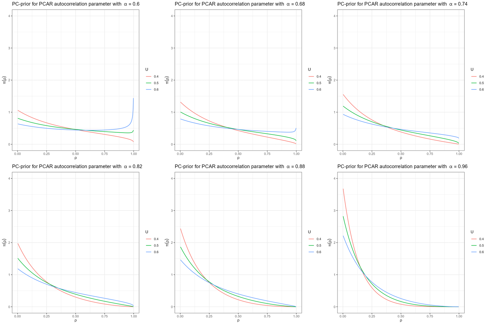
A generalisation of this model is the PCAR (proper CAR), which introduces an autocorrelation parameter \(\alpha\):

\[\begin{equation} z_i \mid z_{-i} \sim N \left( \sum_{j=1}^n \alpha \frac{w_{ij}}{d_i} z_j \,, \frac{\sigma^2}{d_i}\right) \label{eq:pcar_loc} \end{equation}\]

The R code to implement the PCAR model in R-INLA is in Appendix.

We show the posterior summary for the autocorrelation coefficient.

## Mean            0.82507 
## Stdev           0.1313 
## Quantile  0.025 0.480245 
## Quantile  0.25  0.761958 
## Quantile  0.5   0.860753 
## Quantile  0.75  0.923041 
## Quantile  0.975 0.976918

BYM model

Perhaps, our data are generated by a process dominated by noise. We can thus try a different path: the BYM model. On a preliminary stance, we keep trusting in the accuracy of the Laplace approximation and stick to INLA. On a later stage, it would be more rigorous to compare INLA results to the posteriors of a model estimated with MCMC.

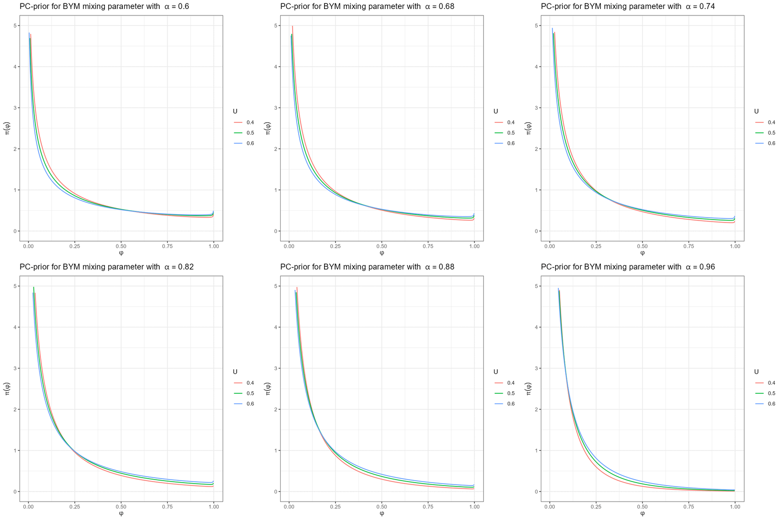
The BYM model we employ follows the parametrisation of (Riebler et al. 2016):

\[\begin{equation} z_i = \sigma \left(\sqrt{\phi} u_i + \sqrt{1-\phi} v_i \right) \label{eq_bym2} \end{equation}\]

where \(u\) is an ICAR field, \(v\) is an IID standard Gaussian white noise i.e. \(v \sim N(0, I)\), and \(\phi\) is a mixing parameter \(\in [0, 1]\).

LCAR model

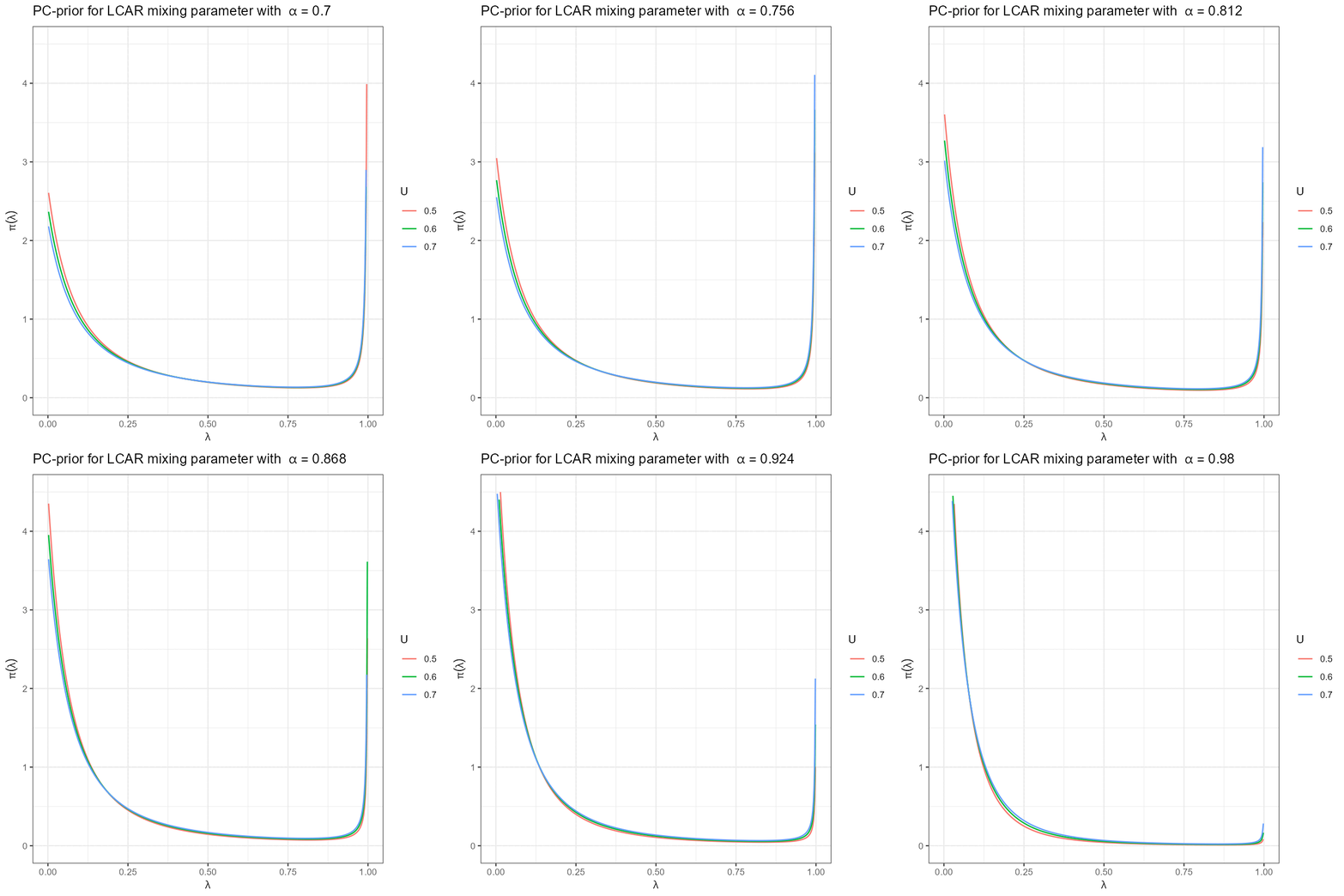
As an alternative to take into account both structured and unstructured latent effects, we also test the Leroux autoregressive model (Leroux, Lei, and Breslow 2000), which we will refer to as LCAR. In this case, the local prior for \(z_i\) is

\[\begin{equation} z_i \mid z_{-i} \sim N \left( \sum_{j=1}^n \frac{\xi w_{ij}}{1 - \xi + \xi d_i} z_j \,, \frac{\sigma^2}{1 - \xi + \xi d_i}\right) \label{eq:leroux_loc} \end{equation}\]

Where \(\xi \in [0, 1]\) is the mixing parameter. A more interesting representation of the Leroux model is the joint prior \[ z \mid \sigma^2, \xi \sim N(0, \sigma^2[\xi R + (1-\xi)I]^{-1}) \] where \(R := D-W\) is the graph Laplacian matrix, \(W\) is the neighbourhood matrix and \(D\) is the corresponding degree matrix.

Comparison

We briefly compare these four through the WAIC (Gelman, Hwang, and Vehtari 2014):

As we can see, models taking into account random noise have a better performance.

Posterior estimates of \(\alpha\) under the BYM model are shown.

Estimations of \(\alpha\) differ from the nonspatial model. For all variables, credibility intervals are wider due to increased uncertainty.

Comments are postponed to the next session.

Lastly, we take a look at model hyperparameters:

## Warning: Use of .data in tidyselect expressions was deprecated in tidyselect 1.2.0.
## ℹ Please use `"Variable"` instead of `.data$Variable`
## This warning is displayed once every 8 hours.
## Call `lifecycle::last_lifecycle_warnings()` to see where this warning was
## generated.

Even though the value of the zero-inflation parameter is low, we can see deep differences in the structure of the latent effects: the precision parameter median of the ZIP model is almost double than under the Poisson model, while the mixing parameter is shrunk.

For completeness, we show the hyperparameters posterior summary also for the Leroux model. The mixing parameter is not directly comparable. Neither does the precision parameter, since only under intrinsic models can the Laplacian matrix be scaled a priori. That being said, we see the difference between the two likelihoods is analogous.

It is, however, worthy noticing how INLA manages to meet the regularity conditions to approximate the CPO more often than in the non-inflated model. Still, CPO must be re-computed manually before employing it as an evaluation metrics:

sum(cav_bym_INLA$cpo$failure)
sum(cav_bym_INLA$cpo$failure > 0)


sum(cav_bym_INLA_ZIP$cpo$failure)
sum(cav_bym_INLA_ZIP$cpo$failure > 0)

sum(cav_leroux_INLA$cpo$failure)
sum(cav_leroux_INLA$cpo$failure > 0)


sum(cav_leroux_INLA_ZIP$cpo$failure)
sum(cav_leroux_INLA_ZIP$cpo$failure > 0)

Lastly, we plot the estimated latent BYM effect under the Poisson model

Spatial regression accounting for underreporting

So far, under-reporting has not been explicitly modelled. Rather, explanatory variables maintained a twofold interpretation as affecting either VAW occurrence, VAW reporting, or both.

Let us consider a regression model in which, for instance, either the incidence of low education or the employment rate are not taken into account for some reason, and compare them with the full model.

As it can be seen, the mean effect of employment rate is shrunk to \(1/10\) of its value under the full model. How can this fact be interpreted? The two explanatory variables have a strong negative correlation (\(-0.64\)), yet their effects on the target variable have the same sign, and removing one (ELL) from the model reduces the expected effect of the other (see ‘full’ versus ‘noELL’). Removing the employment rate, instead, has a milder impact on the expected effect of low education incidence (see ‘full’ versus ‘noER’).

This finding may suggest us that different variables impact different components of the target variable, and perhaps this bifid effect should be modelled separately. We assume these two different components are VAW occurrence and VAW reporting when occurring.

In absence of either validation data, or information on complete-reporting contexts, we can only guess how to partition the effect of explanatory variables between VAW occurrence and reporting.

As an exploratory tool, we rely on a Poisson-logistic model (Stoner, Economou, and Silva 2019), (Arima, Calculli, and Pollice 2025). In brief, we have \[ y_i \sim \mathrm{Poisson(E_i\, \lambda_i \pi_i)} \] Where \(\lambda_i \in \mathbb{R}^{+}\) is the parameter controlling the occurrence of true counts, and \(\pi_i \in [0,1]\) controls for reporting frequency. \(E_i\) is the offset, i.e. the female population aged \(>14\) years. Due to the different domains of \(\pi_i\) and \(\lambda_i\), this parametrisation implies departure from linearity in the predictor.

For clarity, in the following we will denote \(\alpha\) as the \(k+1\) covariate effects entering \(\lambda_i\) and \(\beta\) the \(m+1\) covariate effects entering \(\pi_i\) for two integers \(p\) and \(m\). We would thus have \[ \lambda_i = e^{\displaystyle{\alpha_0 + \alpha_1 X_{i1} + ... + \alpha_p X_{ik}} + z_i} \] And \[ \pi_i = \left(1 + e^{- \displaystyle{(\beta_0 + \beta_1 X_{k+1} + ... + \beta_m X_{i, k+m})}} \right)^{-1} \] Hence the predictor is not linear anymore. \(z_i\) denotes the spatial latent effect, as in earlier section.

As a preliminary modelling and computation attempt we employ the inlabru R package (Lindgren et al. 2024), following the operational (and coding) framework of (Wøllo 2022).

The inlabru R package allows for wrapping of inla() function calls within a more generalised environment, which is extended to nonlinear regression models.

The core idea is to approximate the linear predictor with a linear function of the parameters by a first-order Taylor approximation.

R codes are based on the ones shared by (Wøllo 2022) on this GitHub repo.

We assign the TEP_th_22 and ELL covariates to the underreporting DGP and ER to VAW occurrring DGP. An informative prior is assigned to the intercept \(\beta_0\). The idea is that, when all other effects are zero, \(\pi_i \approx 1/10\).

However, interpreting \(\beta_0\) is limited due to the mutual non-identifiability issue with \(\alpha_0\). Raising the prior mean of \(\beta_0\) would imply a reduction in the posterior mean of \(\alpha_0\), and vice versa.

This is the code to fit a Pogit model given a model for the latent spatial effect:

library(inlabru)

logexpit <- function(x, beta){
  pred <- beta[[1]] +
    rowSums(do.call(cbind, lapply(c(1:length(x)), function(n){
      beta[[n+1]]*x[[n]]
      })))
  return(-log(1+exp(-pred)))
}


cmp_spatial <- function(spatial_expr) {
  f2 <- substitute(spatial_expr)
  f1 <- bquote(
    ~ alpha_0(1) +  
      beta_0(main = 1, model = "linear",
            mean.linear = -2.2,
            prec.linear = 1e+2) +
      myoffset(log(nn), model = "offset") +
      alpha_ELI(ELI) + alpha_PGR(PGR) + alpha_UIS(UIS) + 
      alpha_PDI(PDI) + alpha_ER(ER) +
      beta_TEP(main = 1, model = "linear",
          mean.linear = 0,
          prec.linear = 1e-3) + 
      beta_ELL(main = 1, model = "linear",
          mean.linear = 0,
          prec.linear = 1e-3))
  
  ff <- as.call(c(quote(`+`), f1[[2]], f2))
  final_formula <- as.formula(bquote(~ .(ff)))
  return(final_formula)
}

And this is the code to model the latent spatial effect. We test the ICAR, PCAR, LCAR and BYM models.

cav_bru_basic <- function(model_cmp, verbose = FALSE) {
  terms <- c("alpha_0", "myoffset", "alpha_ELI", "alpha_PGR", "alpha_UIS",
             "alpha_PDI", "alpha_ER",
             paste0("logexpit(x=list(TEP_th_22, ELL) ,",
             "beta = list(beta_0, beta_TEP,  beta_ELL))"))
  
  if (any(grepl("spatial", as.character(model_cmp)))) terms <- c(terms, "spatial")
  
  formula <- as.formula(paste("N_ACC ~", paste(terms, collapse = " + ")))
  
  res <- inlabru::bru(
    components = model_cmp,
    lik = like("poisson", formula = formula,data = dd_con),
    options = list(verbose = verbose, num.threads = 1,
                   control.compute = list(
                     waic = T, cpo = T, dic = T, internal.opt = F)))
  
  return(res)
}

cmp_icar <- cmp_spatial(
  spatial(ID, model = "besag", graph = W_con,
          scale.model = TRUE, 
          hyper = list(prec = list(prior = "pc.prec",
                                                       param = c(1.5, 0.01)))))
#' Here \lambda denotes the rate parameter for the
#' PC prior on the precision:
cmp_pcar <- cmp_spatial(
  spatial(ID, model = PCAR.model(W = W_con, k = 1,
                                 lambda = log(100)/1.5, init = c(0, 4))))

cmp_lcar <- cmp_spatial(
  spatial( ID, model = "besagproper", graph = W_con, 
  hyper = list(prec = list(prior = "pc.prec", param = c(1.5, 0.01)))))

cmp_bym <- cmp_spatial(
  spatial(ID, model="bym2", graph = W_con, 
          scale.model = TRUE, 
          hyper = list(prec = list(prior = "pc.prec", 
                                   param = c(1.5, 0.01)))))
#' Null model
cav_nosp_inlabru <- cav_bru_basic(cmp_spatial(NULL))

#' icar --> simplest, yet not satisfying
cav_icar_inlabru <- cav_bru_basic(cmp_icar)

#' lcar --> better
cav_lcar_inlabru <- cav_bru_basic(cmp_lcar)

#' pcar --> This is going to be obnoxious since verbose = T is mandatory not to make INLA crash :) 
cav_pcar_inlabru <- cav_bru_basic(cmp_pcar, verbose = T)

#' BYM --> best one
cav_bym_inlabru <- cav_bru_basic(cmp_bym)

We compare four competing spatial models and the nonspatial one (Null). As for the case of linear Poisson regression, the best choice appears to be the BYM model.

Pogit model preliminary findings

Model results are generally close to those of the linear Poisson regression (see previous section). We compare covariates effects between the BYM and nonspatial model.

  • TEP_th_22 The effect of the distance from the closest support center remains similar in mean to the nonspatial model and the interpretation should not be altered.

  • ELI: Under the spatial model, the effect of the incidence of low-productivity economic units is shrunk in mean while its variability increases

  • PGR: The association with population growth rate is still positive and significantly \(\neq 0\)

  • UIS: Under the spatial model, the association with the density of productive units appears not significant, due to increased variability

  • ELL: Under the spatial model the association with the incidence of low education levels, instead, is doubled in mean. We interpret this result as a strong potential impact of education on the chance that gender violence is reported

  • PDI: The effect of structural dependency index is utterly negligible.

  • ER: Under the spatial model, the effect associated with employment rate is more than doubled in mean with respect to the nonspatial model. How to interpret this finding? Employment rate is clearly an indicator of economic development, hence the easiest interpretation is that - as it was with ELI under the nonspatial model - in more developed areas there is a higher chance that gender violence is reported.

We also plot the posterior marginal densities of covariate effects under the BYM model.
Estimated covariate effects with the pogit model with BYM latent effect

Estimated covariate effects with the pogit model with BYM latent effect

In the following, posterior summaries of BYM hyperparameters are shown.

cav_bym_inlabru_marginals.var <- unlist(inla.zmarginal(inla.tmarginal(
  fun = function(x) 1/x, marginal =cav_bym_inlabru$marginals.hyperpar[[1]]), silent = T))

hyperpars_bru<- data.frame(rbind(cav_bym_inlabru_marginals.var[c(1,3,5,7)],
                   cav_bym_inlabru$summary.hyperpar[2,c(1,3,4,5)])) %>% 
  dplyr::mutate(Variable =c("Variance", "Mixing")) %>% 
                  dplyr::relocate(.data$Variable, .before = 1) 
rownames(hyperpars_bru) <- NULL
hyperpars_bru
Finally, we plot the estimated latent BYM effect:
Expected BYM field under the pogit model

Expected BYM field under the pogit model

Weakness elements and possible developments

From this preliminary analysis, inference on spatial models is hindered by the dominance of random noise over structured spatial effects. This can be argued from the posterior distribution of the mixing parameter in the BYM model, other than from the low spatial autocorrelation parameter in the PCAR.

This means that only to a small extent the variation in \(y\) not explained by covariates can be explained by spatial structure.

On the other hand, it is difficult to assert all variation not explained by covariates is pure noise, otherwise we would have evidence for the lack of autocorrelation in residuals. We tested the hypothesis of no autocorrelation in GLM residuals by the Moran’s \(I\) test, but in doing so we had to only test the residuals of areas with nonzero counts.

Moreover, spatial models are estimated using the INLA. While this is a broadly employed approach in epidemiology and in disease mapping, so far we did not assess how accurate the Laplace approximation has been.

To do so, we should e.g. rerun the same models using MCMC methods, e.g. using R libraries such as CARBayes, and replicating the same prior structure used.

Perhaps, the biggest INLA-related weakness element is the impossibility to apply LOOCV by means of the CPO. This problematic is stressed out by the high rate of failure in meeting the regularity conditions to compute CPOs, flagged by nonzero values in inla$cpo$failure. This issue could be partially mitigated by zero-inflated Poisson regression.

Lastly, data at our disposal are only informative about the reported violence. Higher occurrence of violence reports from a given territory may thus depend on two factors: either the higher occurrence of violence in that territory, or the ease in reporting violence for the residents, and we can only assume a priori which variables impact on either of these two processes.

For instance, regarding the impact of the distance from support centers, whereas the easiest interpretation is that violence occurrence is underestimated in low-reporting areas, with these data at hand nothing prevents us from suspecting that the placement of support centers is instead at least partially strategic, i.e. the distribution of supporting centers is more dense in areas in which violence occurs, for some reason we don’t know, at a higher frequence.

Our solution to the under-reporting issue has been pogit regression (Stoner, Economou, and Silva 2019), (Arima, Calculli, and Pollice 2025). Until now, we have been avoiding the issue of non-linearity by approximating the linear predictor. Comparison with MCMC-run models would be beneficial to assess how righteous this approximation is.

Appendix: the WAIC

Following (Gelman, Hwang, and Vehtari 2014), the WAIC is given by the sum of two components:

\[ WAIC := 2 \sum_{i=1}^n \mathrm{VAR}[\ln p(y_i |\theta)] - 2 \sum_{j=1}^n \ln \mathbb{E}[p(y_i | \theta)] \] Where \(\theta\) is the full set of model parameters; the variance and the average are computed by integrating over the posterior of \(\theta\). The first addendum denotes the number of free parameters, while the second term is a measure for goodness of fit.

Appendix: R code to implement the PCAR model in INLA

Although it is not readily implemented in R-INLA (the "besagproper" effect is actually the Leroux model) we may base the R code on the `INLAMSM`` package (Palmí-Perales, Gómez-Rubio, and Martinez-Beneito 2021):

inla.rgeneric.PCAR.model <- 
  function (cmd = c("graph", "Q", "mu", "initial", "log.norm.const", 
                                              "log.prior", "quit"), theta = NULL) {
  interpret.theta <- function() {
    alpha <- 1/(1 + exp(-theta[1L])) # alpha modelled in logit scale
    mprec <- sapply(theta[2L], function(x) {
      exp(x)
    })
    PREC <- mprec
    return(list(alpha = alpha, mprec = mprec, PREC = PREC))
  }
  graph <- function() {
    G <- Matrix::Diagonal(nrow(W), 1) + W
    return(G)
  }
  Q <- function() {
    param <- interpret.theta()
    Q <- param$PREC * 
      (Matrix::Diagonal(nrow(W), apply(W, 1, sum)) - param$alpha * W)
    return(Q)
  }
  mu <- function() {
    return(numeric(0))
  }
  log.norm.const <- function() {
    val <- numeric(0)
    return(val)
  }
  log.prior <- function() {
    param <- interpret.theta()
    val <- -theta[1L] - 2 * log(1 + exp(-theta[1L]))
    # # PC prior
    val <- val + log(lambda/2) - theta[2L]/2 - (lambda * exp(-theta[2L]/2))
    # # Gamma(1, 5e-5), default prior:
    #val <- val + dgamma(exp(theta[2L]), shape = 1, rate = 5e-5, log = T) + theta[2L]
    # # Uniform prior on the standard deviation
    #val <- val - sum(theta[2L])/2 - k * log(2)
    return(val)
  }
  initial <- function() {
    return(c(0, 4))
  }
  quit <- function() {
    return(invisible())
  }
  if (as.integer(R.version$major) > 3) {
    if (!length(theta)) 
      theta = initial()
  }
  else {
    if (is.null(theta)) {
      theta <- initial()
    }
  }
  val <- do.call(match.arg(cmd), args = list())
  return(val)
  }

PCAR.model <- function(...) INLA::inla.rgeneric.define(inla.rgeneric.PCAR.model, ...)

Bibliography

Arima, Serena, Crescenza Calculli, and Alessio Pollice. 2025. “A Zero-Inflated Poisson Spatial Model with Misreporting for Wildfire Occurrences in Southern Italian Municipalities.” Environmetrics 36 (1): e2853.
Gelman, Andrew, Jessica Hwang, and Aki Vehtari. 2014. “Understanding Predictive Information Criteria for Bayesian Models.” Statistics and Computing 24 (6): 997–1016. https://doi.org/10.1007/S11222-013-9416-2.
Leroux, Brian G., Xingye Lei, and Norman Breslow. 2000. “Estimation of Disease Rates in Small Areas: A New Mixed Model for Spatial Dependence.” In Statistical Models in Epidemiology, the Environment, and Clinical Trials, edited by M. Elizabeth Halloran and Donald Berry, 179–91. New York, NY: Springer New York. https://doi.org/https://doi.org/10.1007/978-1-4612-1284-3_4.
Lindgren, Finn, Fabian Bachl, Janine Illian, Man Ho Suen, Håvard Rue, and Andrew E Seaton. 2024. “Inlabru: Software for Fitting Latent Gaussian Models with Non-Linear Predictors.” arXiv Preprint arXiv:2407.00791. https://doi.org/https://doi.org/10.48550/arXiv.2407.00791.
Palmí-Perales, Francisco, Virgilio Gómez-Rubio, and Miguel A. Martinez-Beneito. 2021. “Bayesian Multivariate Spatial Models for Lattice Data with INLA.” Journal of Statistical Software 98 (2): 1–29. https://doi.org/10.18637/jss.v098.i02.
Riebler, Andrea, Sigrunn H Sørbye, Daniel Simpson, and Håvard Rue. 2016. “An Intuitive Bayesian Spatial Model for Disease Mapping That Accounts for Scaling.” Statistical Methods in Medical Research 25 (4): 1145–65.
Stoner, Oliver, Theo Economou, and Gabriela Drummond Marques da Silva. 2019. “A Hierarchical Framework for Correcting Under-Reporting in Count Data.” Journal of the American Statistical Association.
Van Niekerk, Janet, Elias Krainski, Denis Rustand, and Haavard Rue. 2023. “A New Avenue for Bayesian Inference with INLA.” Computational Statistics and Data Analysis 181. https://doi.org/10.1016/j.csda.2023.107692.
Wøllo, Sara E. 2022. “Correcting for Under-Reporting of Violence Against Women in Italy Using INLA.” NTNU Open. https://hdl.handle.net/11250/3026838.